6 Making Predictions
To make predictions, I will use the retained iterations from the gri_stanfit object. Alternatively, I could use the means of the posterior distributions to calculate a single lambda for each score within each game. These lambda values could then be used to generate a sample of scores which could be used to predict the outcome of the game. However, this approach would ignore the uncertainty in the parameter estimates. A better solution would be to calculate lambda values at each iteration of the chain, using the current estimates of the parameters. Thus, at each iteration, it is possible to simulate a score for each team at each iteration, creating a posterior distribution for the score of each game.
6.1 Predict individual games
First, I will extract the parameters we need from the fitted model, and load in the team codes associated with each team.
model_params <- rstan::extract(gri_stanfit, pars = c("mu", "eta", "alpha",
  "delta", "sigma_g"))
load("_data/team_counts.rda")
I then use the predict_games function (see Appendix D.1) to predict the outcome of a game between any two teams included in the model. For example, we can predict the winner of a game between Barcelona and Real Madrid played in Barcelona.
library(dplyr)
library(ggplot2)
library(purrr)
prediction <- predict_game(home = "Barcelona", away = "Real Madrid",
  neutral = FALSE, visualize = TRUE, team_codes = team_counts,
  chains = model_params)

prediction$predictions %>%
  select(Club = club, `Expected Goals` = expected_goals,
    `Win Probability` = prob_win, `Tie Probability` = prob_tie) %>%
  knitr::kable(caption = "Prediction for Real Madrid at Barcelona",
align = "c", digits = 3)| Club | Expected Goals | Win Probability | Tie Probability |
|---|---|---|---|
| Barcelona | 2.76 | 0.591 | 0.171 |
| Real Madrid | 1.74 | 0.238 | 0.171 |
Because I specified visualize = TRUE in the call to predict_game we can use the multiplot function (Appendix D.2) to visualize the range of possible outcomes from the posteriors.
library(grid)
multiplot(plotlist = prediction$plots, cols = 2)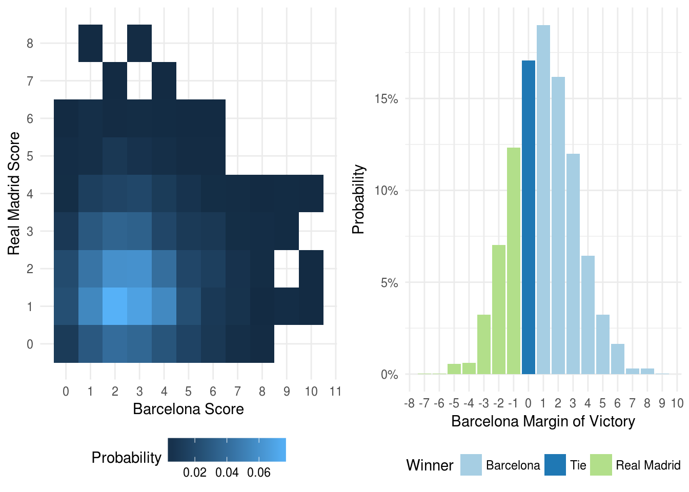
Figure 6.1: Visualizations for Real Madrid at Barcelona
6.2 Predict domestic leagues
To predict entire leagues, I follow the same general process, simulating an outcome for each retained iteration of the chain. The difference for leagues is that instead of simulating a single game at each iteration, we simulate the remainder of the league season, and calculate the league winner. This is all done by the predict_league function (Appendix D.3).
In order to simulate these outcome, I’ll first need to load in the full data set that includes future games
library(lubridate)
library(rvest)
library(tidyr)
library(scales)

load("_data/full_data.rda")
load("_data/club_rankings.rda")
Then, I can use the predict_league function to get championship probabilities for each league.
6.2.1 English Premier League
predict_league(league = "Premier League", games = full_data,
  chains = model_params, team_codes = team_counts) %>%
  left_join(select(club_rankings, club, exp_offense, exp_defense),
    by = "club") %>%
  arrange(desc(champ_pct)) %>%
  mutate(champ_pct = percent(ifelse(is.na(champ_pct), 0, champ_pct))) %>%
  select(Club = club, Offense = exp_offense, Defense = exp_defense,
    `Expected Points` = sim_points, `Championship Probability` = champ_pct) %>%
  knitr::kable(caption = "Premier League Championship Probabilities",
align = "c", digits = 2)| Club | Offense | Defense | Expected Points | Championship Probability |
|---|---|---|---|---|
| Chelsea | 1.93 | 0.78 | 90.2 | 92.5% |
| Tottenham Hotspur | 1.81 | 0.72 | 84.6 | 7.5% |
| Liverpool | 1.73 | 0.81 | 75.2 | 0.0% |
| Manchester City | 1.80 | 0.81 | 74.7 | 0.0% |
| Manchester United | 1.54 | 0.69 | 71.1 | 0.0% |
| Arsenal | 1.90 | 0.91 | 69.5 | 0.0% |
| Everton | 1.41 | 0.90 | 62.4 | 0.0% |
| West Bromwich Albion | 1.09 | 0.98 | 47.9 | 0.0% |
| Southampton | 1.08 | 0.88 | 46.9 | 0.0% |
| AFC Bournemouth | 1.25 | 1.19 | 45.4 | 0.0% |
| Leicester City | 1.24 | 1.06 | 45.0 | 0.0% |
| Stoke City | 1.02 | 1.04 | 43.0 | 0.0% |
| Watford | 1.00 | 1.10 | 42.9 | 0.0% |
| Burnley | 1.00 | 0.95 | 43.4 | 0.0% |
| West Ham United | 1.13 | 1.20 | 41.7 | 0.0% |
| Crystal Palace | 1.17 | 1.10 | 40.8 | 0.0% |
| Hull City | 1.13 | 1.13 | 37.7 | 0.0% |
| Swansea City | 1.23 | 1.20 | 36.2 | 0.0% |
| Middlesbrough | 0.99 | 0.92 | 30.6 | 0.0% |
| Sunderland | 0.81 | 1.15 | 23.8 | 0.0% |
6.2.2 French Ligue 1
predict_league(league = "Ligue 1", games = full_data,
  chains = model_params, team_codes = team_counts) %>%
  left_join(select(club_rankings, club, exp_offense, exp_defense),
    by = "club") %>%
  arrange(desc(champ_pct)) %>%
  mutate(champ_pct = percent(ifelse(is.na(champ_pct), 0, champ_pct))) %>%
  select(Club = club, Offense = exp_offense, Defense = exp_defense,
    `Expected Points` = sim_points, `Championship Probability` = champ_pct) %>%
  knitr::kable(caption = "Ligue 1 Championship Probabilities",
align = "c", digits = 2)| Club | Offense | Defense | Expected Points | Championship Probability |
|---|---|---|---|---|
| AS Monaco | 2.07 | 0.92 | 91.8 | 95.6% |
| Paris Saint-Germain | 1.99 | 0.73 | 87.3 | 4.4% |
| Nice | 1.28 | 0.92 | 81.1 | 0.0% |
| Lyon | 1.62 | 0.99 | 62.8 | 0.0% |
| Bordeaux | 1.16 | 1.03 | 60.1 | 0.0% |
| Marseille | 1.31 | 0.97 | 60.0 | 0.0% |
| St Etienne | 0.91 | 0.85 | 53.3 | 0.0% |
| Nantes | 0.88 | 1.09 | 51.1 | 0.0% |
| Stade Rennes | 0.85 | 1.07 | 47.5 | 0.0% |
| Guingamp | 1.06 | 1.12 | 48.9 | 0.0% |
| Lille | 0.93 | 0.98 | 47.0 | 0.0% |
| Toulouse | 0.99 | 0.91 | 47.3 | 0.0% |
| Montpellier | 1.14 | 1.32 | 42.3 | 0.0% |
| Angers | 1.00 | 1.07 | 42.8 | 0.0% |
| Metz | 0.89 | 1.39 | 41.8 | 0.0% |
| Lorient | 1.08 | 1.38 | 38.0 | 0.0% |
| Dijon FCO | 1.08 | 1.18 | 36.8 | 0.0% |
| Caen | 0.92 | 1.41 | 35.4 | 0.0% |
| AS Nancy Lorraine | 0.80 | 0.99 | 35.0 | 0.0% |
| Bastia | 0.77 | 1.16 | 33.3 | 0.0% |
6.2.3 German Bundesliga
predict_league(league = "Bundesliga", games = full_data,
  chains = model_params, team_codes = team_counts) %>%
  left_join(select(club_rankings, club, exp_offense, exp_defense),
    by = "club") %>%
  arrange(desc(champ_pct)) %>%
  mutate(champ_pct = percent(ifelse(is.na(champ_pct), 0, champ_pct))) %>%
  select(Club = club, Offense = exp_offense, Defense = exp_defense,
    `Expected Points` = sim_points, `Championship Probability` = champ_pct) %>%
  knitr::kable(caption = "Bundesliga Championship Probabilities",
align = "c", digits = 2)| Club | Offense | Defense | Expected Points | Championship Probability |
|---|---|---|---|---|
| Bayern Munich | 2.13 | 0.70 | 80.1 | 100% |
| RB Leipzig | 1.43 | 0.87 | 66.8 | 0% |
| TSG Hoffenheim | 1.48 | 0.89 | 62.6 | 0% |
| Borussia Dortmund | 1.83 | 0.91 | 63.0 | 0% |
| Hertha Berlin | 1.10 | 0.91 | 50.6 | 0% |
| Werder Bremen | 1.35 | 1.20 | 47.9 | 0% |
| SC Freiburg | 1.09 | 1.25 | 47.0 | 0% |
| FC Cologne | 1.18 | 0.95 | 46.6 | 0% |
| Borussia Monchengladbach | 1.30 | 0.99 | 47.6 | 0% |
| Schalke 04 | 1.37 | 0.88 | 46.6 | 0% |
| Eintracht Frankfurt | 0.95 | 0.87 | 45.2 | 0% |
| Bayer Leverkusen | 1.26 | 1.04 | 40.2 | 0% |
| FC Augsburg | 0.99 | 1.15 | 37.3 | 0% |
| Mainz | 1.17 | 1.15 | 36.9 | 0% |
| VfL Wolfsburg | 0.92 | 1.07 | 36.5 | 0% |
| Hamburg SV | 0.96 | 1.26 | 36.4 | 0% |
| FC Ingolstadt 04 | 0.95 | 1.16 | 32.4 | 0% |
| SV Darmstadt 98 | 0.84 | 1.29 | 25.9 | 0% |
6.2.4 Italian Serie A
predict_league(league = "Serie A", games = full_data,
  chains = model_params, team_codes = team_counts) %>%
  left_join(select(club_rankings, club, exp_offense, exp_defense),
    by = "club") %>%
  arrange(desc(champ_pct)) %>%
  mutate(champ_pct = percent(ifelse(is.na(champ_pct), 0, champ_pct))) %>%
  select(Club = club, Offense = exp_offense, Defense = exp_defense,
    `Expected Points` = sim_points, `Championship Probability` = champ_pct) %>%
  knitr::kable(caption = "Serie A Championship Probabilities",
align = "c", digits = 2)| Club | Offense | Defense | Expected Points | Championship Probability |
|---|---|---|---|---|
| Juventus | 1.66 | 0.64 | 92.0 | 99.2% |
| AS Roma | 1.75 | 0.87 | 82.3 | 0.7% |
| Napoli | 1.76 | 0.92 | 81.7 | 0.1% |
| Lazio | 1.49 | 0.92 | 74.0 | 0.0% |
| Atalanta | 1.37 | 0.93 | 71.0 | 0.0% |
| AC Milan | 1.24 | 0.95 | 64.5 | 0.0% |
| Internazionale | 1.44 | 1.13 | 62.2 | 0.0% |
| Fiorentina | 1.36 | 1.06 | 60.9 | 0.0% |
| Torino | 1.51 | 1.14 | 54.4 | 0.0% |
| Sampdoria | 1.05 | 0.99 | 50.8 | 0.0% |
| Udinese | 1.08 | 1.09 | 48.1 | 0.0% |
| Cagliari | 1.20 | 1.32 | 45.6 | 0.0% |
| Chievo Verona | 1.01 | 1.09 | 45.7 | 0.0% |
| Sassuolo | 1.15 | 1.16 | 43.9 | 0.0% |
| Bologna | 1.00 | 1.06 | 43.0 | 0.0% |
| Genoa | 0.97 | 1.29 | 34.0 | 0.0% |
| Empoli | 0.75 | 1.12 | 33.4 | 0.0% |
| Crotone | 0.83 | 1.15 | 28.9 | 0.0% |
| Palermo | 0.83 | 1.37 | 23.7 | 0.0% |
| US Pescara | 0.89 | 1.44 | 18.5 | 0.0% |
6.2.5 Spanish La Liga
predict_league(league = "La Liga", games = full_data,
  chains = model_params, team_codes = team_counts) %>%
  left_join(select(club_rankings, club, exp_offense, exp_defense),
    by = "club") %>%
  arrange(desc(champ_pct)) %>%
  mutate(champ_pct = percent(ifelse(is.na(champ_pct), 0, champ_pct))) %>%
  select(Club = club, Offense = exp_offense, Defense = exp_defense,
    `Expected Points` = sim_points, `Championship Probability` = champ_pct) %>%
  knitr::kable(caption = "La Liga Championship Probabilities",
align = "c", digits = 2)| Club | Offense | Defense | Expected Points | Championship Probability |
|---|---|---|---|---|
| Barcelona | 2.30 | 0.83 | 87.9 | 65.6% |
| Real Madrid | 2.18 | 0.94 | 87.6 | 34.4% |
| Atletico Madrid | 1.43 | 0.67 | 77.0 | 0.0% |
| Sevilla FC | 1.33 | 0.94 | 72.8 | 0.0% |
| Villarreal | 1.15 | 0.82 | 67.1 | 0.0% |
| Athletic Bilbao | 1.21 | 0.93 | 66.1 | 0.0% |
| Real Sociedad | 1.29 | 1.04 | 64.9 | 0.0% |
| Eibar | 1.26 | 1.03 | 57.2 | 0.0% |
| Espanyol | 1.09 | 0.98 | 54.8 | 0.0% |
| Alavés | 0.97 | 0.86 | 52.4 | 0.0% |
| Celta Vigo | 1.28 | 1.03 | 48.2 | 0.0% |
| Málaga | 1.08 | 1.15 | 45.1 | 0.0% |
| Valencia | 1.22 | 1.25 | 44.4 | 0.0% |
| Las Palmas | 1.27 | 1.32 | 42.3 | 0.0% |
| Real Betis | 0.94 | 1.17 | 40.2 | 0.0% |
| Deportivo La Coruña | 1.02 | 1.19 | 35.6 | 0.0% |
| Leganes | 0.83 | 1.12 | 33.5 | 0.0% |
| Sporting Gijón | 0.96 | 1.35 | 27.6 | 0.0% |
| Granada | 0.78 | 1.40 | 22.6 | 0.0% |
| Osasuna | 0.91 | 1.51 | 21.8 | 0.0% |
6.3 UEFA Champions League
Simulating the UEFA Champions League is very similar to the process used for simulating the domestic leagues. At each retained iteration of the MCMC chain, I simulate the remainder of the Champions League matches. Because there isn’t a true bracket, and the opponents are drawn randomly before each round, I first define the current match-ups.
matchups <- list(
  c("Real Madrid", "Atletico Madrid"),
  c("AS Monaco", "Juventus")
)
I can then use the predict_ucl function (Appendix D.4) to calculate the probability of each team advancing to each subsequent round.
predict_ucl(matchups = matchups, games = full_data, chains = model_params,
  team_codes = team_counts) %>%
  left_join(select(club_rankings, club, exp_offense, exp_defense),
    by = c("Club" = "club")) %>%
  arrange(desc(Champion)) %>%
  mutate(Quarterfinals = percent(Quarterfinals),
    Semifinals = percent(Semifinals), Final = percent(Final),
    Champion = percent(Champion)) %>%
  select(Club, Offense = exp_offense, Defense = exp_defense, Quarterfinals,
    Semifinals, Final, Champion) %>%
  knitr::kable(caption = "UEFA Champions League Probabilities",
align = "c", digits = 2)| Club | Offense | Defense | Quarterfinals | Semifinals | Final | Champion |
|---|---|---|---|---|---|---|
| Juventus | 1.66 | 0.64 | 100% | 100% | 90.5% | 48.7% |
| Real Madrid | 2.18 | 0.94 | 100% | 100% | 94.7% | 43.6% |
| AS Monaco | 2.07 | 0.92 | 100% | 100% | 9.5% | 5.0% |
| Atletico Madrid | 1.43 | 0.67 | 100% | 100% | 5.3% | 2.7% |